Why do we minimize the mean squared error?

One of the first topics that one encounters when learning machine learning is linear regression. It’s usually presented as one of the simplest algorithms for regression. In my case, when I studied linear regression - back in the days during my physics degree - I was told that linear regression tries to find the line that minimizes the sum of squared distances to the data. Mathematically this is $y^{p} = ax + b$, where $x$ is the independent variable that will be used to predict $y^t$, $y^p$ is the corresponding prediction, and $a$ and $b$ are the slope and intercept. For the sake of simplicity let’s assume that $x\in \mathbb{R}$ and $y\in \mathbb{R}$. The quantity that we want to minimize - aka the loss function - is

The intuition behind this loss is that we want to penalize more big errors than small errors, and that’s why we’re squaring the error term. With this particular choice of the loss functions, it’s better to have 10 errors of 1 unit than 1 error of 10 units - in the first case we would increase the loss in 10 squared units, while in the second case we would increase it by 100 squared units.

However, while this is intuitive, it also seems quite arbitrary. Why using the square function and not the exponential function or any other function with similar properties? The answer is that the choice of this loss function is not that arbitrary, and it can be derived from more fundamental principles. Let me introduce you maximum likelihood estimation!

Maximum Likelihood Estimation

In this section, I’ll present maximum likelihood estimation, one of my favorite techniques in machine learningt, and I’ll show how can we use this technique for statistical learning.

Basics

First of all some theory. Consider a dataset $\mathbf{X} = {x_1, …, x_n}$ of $n$ data points drawn independently from the distribution $p_{\text{real}}(x)$. We have also the distribution $p_{\text{model}}(\theta, x)$, which is indexed by the parameter $\theta$. This means that for each $\theta$ we have a different distribution. For example, one could have $p_{\text{model}}(\theta, x) = \theta e^{-\theta x}$, aka the exponential distribution.

The problem we want to solve is to find $\theta^* $ that maximizes the probability of $\mathbf{X}$ being generated by $p_{\text{model}}(\theta^*, x)$. This is, for all the possible $p_{\text{model}}$ distributions, which is the one that most likely could have generated $\mathbf{X}$. This can be formalized as

and since the observations from $\mathbf{X}$ are extracted independently we can rewrite the equation as

While this equation is completely fine from a mathematical point of view, there are some numerical problems with it. In particular, we’re multiplying probability densities, and densities can be very small sometimes, so the total product can have underflow problems - ie: we can’t represent the value with the precision of our CPU. The good news is that this problem can be overcome with a simple trick: just apply $\log$ to the product and convert the product to a sum.

Since logarithm is a monotonic increasing function, this trick doesn’t change the argmax.

Example

Let’s work out an example to see how one can use this technique in a real problem. Imagine you have two blobs of data that follow a gaussian distribution - or at least that is what you suspect - and you want to find the most probable center of these blobs.

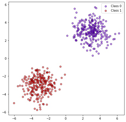
Our hypothesis is that these distributions follow a Gaussian distribution with unit covariance, ie: $\pmb{\Sigma} = [[1, 0], [0, 1]]$. Therefore, we want to maximize

where $\pmb{\theta} = (\pmb\theta_1, \pmb\theta_2)$, and $\pmb\theta_1$ and $\pmb\theta_2$ are the centers of the distributions.

Using the following snippet one can get the most plausible centers according to MLE

from scipy.optimize import minimize
import numpy as np
class Problem:
    def __init__(self, x1, x2):
        self.x1 = x1
        self.x2 = x2
    def loss(self, x):
        mu1 = (x[0], x[1])
        mu2 = (x[2], x[3])
        log_likelihood = (- 1/2 * np.sum((self.x1 - mu1)**2) 
                          - 1/2 * np.sum((self.x2 - mu2)**2))
        # adding - to make function minimizable
        return - log_likelihood 
# x1 and x2 are arrays with the coordinates 
# of points for blob 1 and 2 respectively.
p = Problem(x1=x1, x2=x2) 
res = minimize(p.loss, x0=(0, 0, 0, 0))
print(res.x)

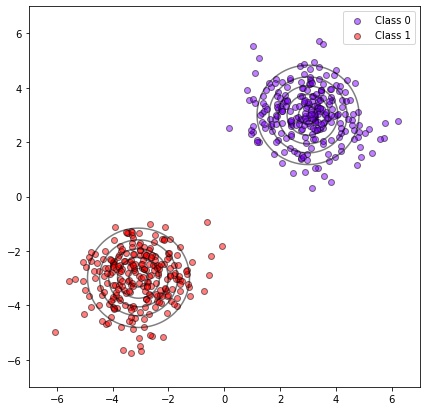
In the following figure, we can see the most plausible generating distributions according to MLE. In this specific case, the real centers are in (3, 3) and (-3, -3), and the optimal found values are (3.003, 3.004) and (-3.074, -2.999) respectively, so the method seems to work.

Using MLE for predictions

In the last section, we have seen how to use MLE to estimate the parameters of a distribution. However, the same principle can be extended to predict $y$ given $x$, using the conditional probability $P(\mathbf{Y} \vert \mathbf{X}; \theta)$. In this case, we want to estimate the parameters of our model that better predict $y$ given $x$, this is

and using the same tricks as before

Now, the process that generates the real data can be written as $y = f(x) + \epsilon$, where $f(x)$ is the function we want to estimate, and $\epsilon$ is the intrinsic noise of the process. Here we are assuming that $x$ has enough information to predict $y$, and no amount of extra information could help us in predicting noise $\epsilon$. One common assumption is that this noise is normally distributed, ie: $\epsilon \sim \mathcal{N}(0, \sigma^2)$. The intuition behind this choice is that even knowing all the variables that describe the system, you will always have some noise, and this noise usually follows a Gaussian distribution. For example, if you take the distribution of heights of all the women, with the same age, and in the same town, you are going to find a normal distribution.

Therefore, a good choice for the conditional probability for our case is

where $\hat{f}(x)$ is our model and is indexed by $\theta$. This means that our model $f$ will predict the mean of the Gaussian.

Plugging now the conditional probability in the equation for $\theta^*$ we get

where $y_i^p$ is the output of our regression model for input $x_i$. Notice that both $n$ and $\sigma$ are constant values, so we can drop them from the equation. Therefore the function that we want to solve is

which is the same as minimizing the loss function $\mathcal{L}$!

But why? Our intuition behind the loss function was that it penalizes big over small errors, but what does this have to do with conditional probabilities and normal distributions?

The point is that extreme values are very unlikely in a normal distribution, so they will contribute negatively to the likelihood. For example, for $p(x) = \mathcal{N}(x; 0, 1)$, $\log p(1) \approx -1.42$, while $\log p(10) \approx -50.92$. Therefore, when maximizing the likelihood we’ll prefer values of $\theta$ that avoid extreme values of $(y^t - y^p)^2$. So the answer to the question Why should we minimize MSE? is Because we’re assuming the noise is normally distributed.

Conclusions

We just saw that minimizing the squared error is not an arbitrary choice but it has a theoretical foundation. We also saw that it comes from assuming that the noise is distributed normally. The same procedure we studied in this post can be used to derive multiple results, for example: the unbiased estimator of the variance, Viterbi Algorithm, logistic regression, machine learning classification, and a lot more.