How far can you jump from a swing?

Discussion on HackerNews.
Some people pointed out some flaws in my modelling (eg: assuming zero distance from swing to floor) which I’ve tried to fix. The original maximum distance estimation was around $1m$.

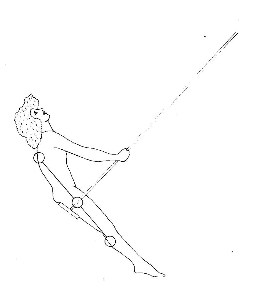
This summer I’ve spent an absurd amount of time reading and learning about the physics of swings. Yes, you read it right, I’ve been learning about the physical processes that happen when a kid is playing with a swing in the park. Blame it on my kids and the countless hours spent enjoying these moments with them. In particular, I read about the physics of pumping a swing and about the physics of jumping from a swing. Amidst my deep dive into swing physics, I came up with a new Olympic sport in which you start seated on a swing with length $L$, your feet comfortably touching the ground. As a countdown of $T$ seconds commences, you embark on the art of swing-pumping. Your challenge is to execute a skillful leap before the countdown reaches zero. With your jump, you travel a distance $d$ from your initial point, aiming to achieve the greatest possible $d$.

The question is then, which is the best method to maximize $d$?

Before I present you with the answer to the question I’ll summarize the learnings I got from reading about the physics of a swing. As usual, you can find all the code I used for this post in my repo.

Notice that ¹ and ² answer a very similar question: what is the optimal time $t$ to jump off, so as to reach farthest. However, these references do not deal with the pumping of a swing, they just assume that you start swinging at some angle $\lambda$ and jump at an angle $\phi$, without pumping the swing at any point. Solving this problem is interesting, but I think it’s more exciting to solve it when the person swinging can control the system. This makes it feel more like a real game that you can play in a park or at the Olympic Games.

Pumping a swing

There are several papers about the pumping of a swing ³, ⁴, and ⁵ and much more. In this section, I’ll focus in particular on ⁴.

The model for a swing I’ll use is a rigid dumbbell made up of three masses, suspended by a rigid rod of length $l_1$ attached to the middle mass $m_1$. The distances from $m_1$ to the other masses $m_2$ and $m_3$ are $l_2$ and $l_3$ respectively. The angle of the rod $l_1$ with the vertical is $\phi$ and the angle of the dumbbell with the rod is $\theta$. In the next figure, you can see a diagram of the system

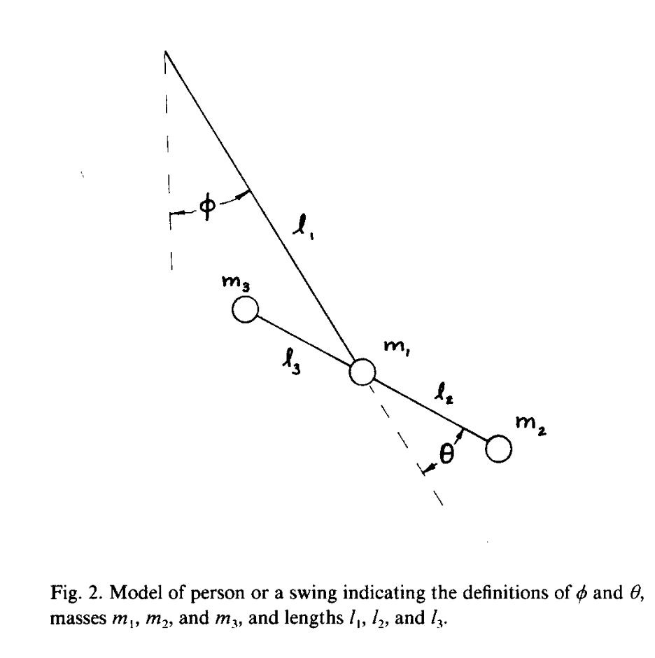
The Lagrangian of this system is

where $M = m_1 + m_2 + m_3$, $N = m_3 l_3 - m_2 l_2$, $I_1 = M l_1^2$, and $I_2 = m_2 l_2^2 + m_3 l_3^2$. Therefore, the Lagrange’s equation for $\phi$ is

The paper proceeds by assuming the swinger pumps the swing by forcing $\theta(t) = \theta_0 \cos(\omega t)$, where $\omega$ is the natural angular frequency of the pendulum. Then, they show that there are two regimes, one where $\phi < \phi_{\text{crit}}$ where the movement is like an harmonic driven oscillator, and another one where $\phi > \phi_{\text{crit}}$ where the movement is an harmonic oscillator with parametric terms. They then analyze the different regimes and solve their equations. In summary, they show that for small amplitudes the swing follows the equation

where

The differential equation has the solution

which looks like for small $t$

This solution is good enough for our approach since I assume $T$ to be small enough to avoid the swinger pumping the swing to big $\phi$ values.

Jumping from a swing

Now let’s study how should a swinger jump from a swing to maximize the traveled distance. The analysis presented here is based on the work of Jason Cole ¹ and Hiroyuki Shima ². Notice that the naive solution of jumping at $\phi=\pi/4$ is not optimal. For instance, imagine a swing that oscillates in the range $\pm \pi/4$, then it’s clear that jumping at $\pi/4$ is suboptimal since the swinger will start its flight with a speed of zero.

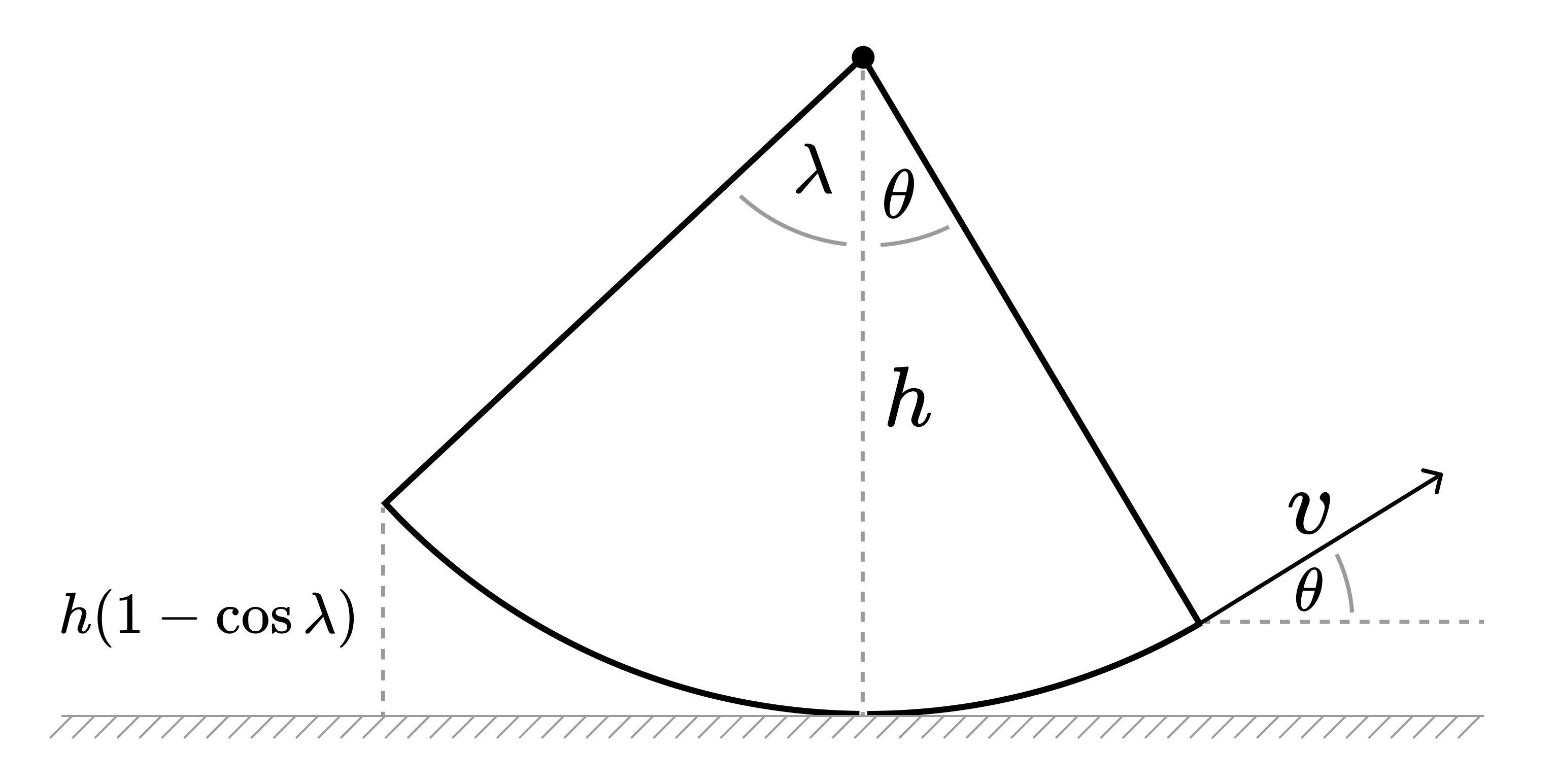
Notice I’m adding a new variable $h$ that represents the distance from the swing to the ground. This variable is not present on Jason’s blog but it’s on Hiroyuki paper. Once you jump from the swing, the equations of motion for the horizontal and the vertical directions are

Now, we can compute the total flight time by solving $y(t_{\text{flight}})=0$ and then compute the flight distance as $d = x(t_{\text{flight}})$. The flight time is then

now notice that only the positive root has physical meaning (we don’t want negative times), so the distance is

Putting everything together

We have now all the pieces we need to solve the problem. On one hand, we can compute the swinger angle $\phi$ for any given $t$, and we can also compute the distance that the swinger will travel when leaving the swing at an angle $\phi$.

Notice that to compute $d$ we need to know $v$. In other sources that study this problem, they get $v$ by using energy conservation, however, in our case, we know $\phi(t)$ and we can get the initial velocity after leaving the swing as $v(t) = l_1 \frac{d}{dt} \phi(t)$

Now, putting everything together we have this set of equations

To compute $d(t)$ we just need to compute $\phi(t)$ and $v(t)$ and substitute the values in the first equation. I’ll use the following constants: $M=1$, $m_1=0.4M$, $m_2 = 0.2M$, $m_3 = 0.4M$, $l_1 = 2$, $l_2 = 0.4$, $l_3 = 0.4$, $h=l_3$, $\theta_0=1$, $g= 9.8$, $T=2 \pi \sqrt{l1 / g}$, and $\omega= 2\pi/T$

With these parameters, we can now plot the traveled distance as a function of the jumping time.

Let’s remember that we’re interested in the optimal jumping time $t^*$ for a given maximum time $T$. To do so we just need to fix a time $T$ and find at which $t^* < T$ the distance $d(t)$ is maximized. I did that numerically and plotted the results in the next image

Of course, the optimal jumping time follows a ladder-like curve. This is because you’re not interested in jumping backward, and sometimes it’s better to jump some seconds before $T$ than to wait for $T$ and find yourself in a worse position.

Finally, we can get also the maximum traveled distance as a function of $T$.

For example, if $T=20s$, which seems like a reasonable value to make the sport interesting, one would expect to achieve $d\approx 2m$.

Conclusion

Well, that’s all for today. In this post, I’ve presented a new Olympic sport that consists of pumping on a swing during a given amount of time and then jumping and trying to achieve the maximum distance. With the parameters used in my simulations, I would expect the world record to be around two meters.

The analysis presented here is full of simplifications. Here I list some of the ones I’m aware of

• The swinger model is oversimplified. For instance, authors in ⁵ present a model which is more accurate than the one used here. However, I wanted to keep the analysis “simple”.
• The swinger is assumed to operate in the regime of small $\phi$, which allows us to use an analytical equation for $\phi(t)$. However, an experimented swinger could achieve big oscillation angles in a short amount of time, and then our simplification wouldn’t be valid anymore.
• As a good physicist I’ve neglected any kind of friction (swing-rod, swinger-air, etc.).

Even with all this simplification, I think the analysis stills bring some light to the problem of maximizing the flight distance. Now, the only step still missing is the experimental one: go to a park and try to beat the theoretical maximum distance. According to my numbers, you wouldn’t be able to beat the 2-meter mark.

All of this reminds me of the anecdote of the mathematician and his wife moving a sofa. The mathematician spent a lot of time computing if it was possible to move the sofa from one room to the other, and finally proved it was impossible. Then he went to show it to his wife, which had already moved the sofa to the other room. So I’m pretty sure that it’s going to be possible to beat my theoretical maximum distance. Unfortunately, I don’t have a swing near me right now, so I’ll have to wait until the next visit to the park.

Appendix 1: optimal distribution of masses

Some days after publishing this post I started wondering which was the combination of masses $m_1$, $m_2$, and $m_3$ that allowed for the best results, aka how should a Swing Jumping world champion look like. To do so I have fixed all the parameters except the masses, and I’ve forced $1 = m_1 + m_2 + m_3$ since the behavior of the system is independent of the total mass $M$.

In the next plot we see how the maximum distance depends on $m_2$ and $m_3$. The red star shows where the combination of masses that maximized the distance.

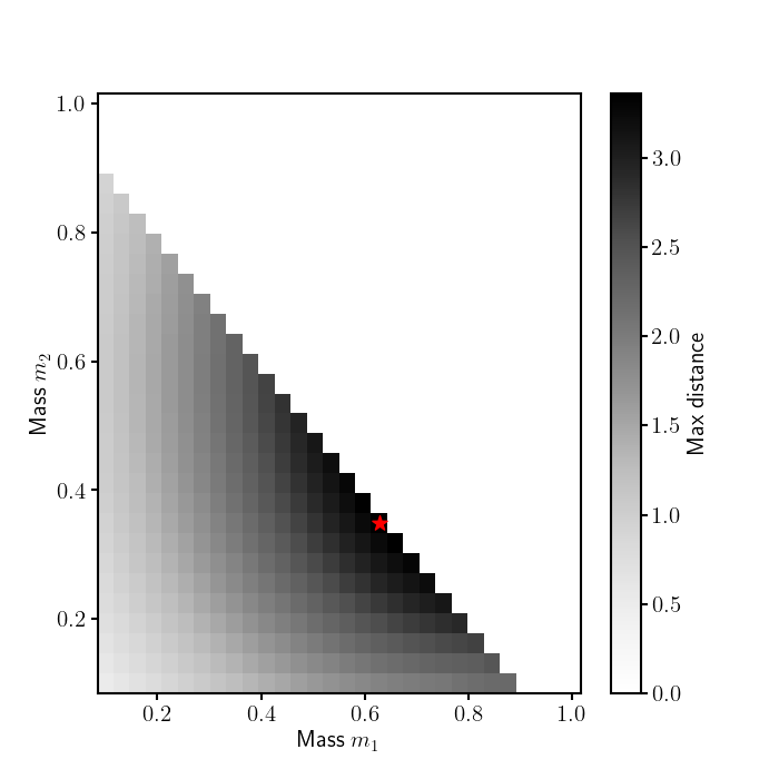
The best combination of masses is $m_1=0$, $m_2 \approx 0.625$ and $m_3 \approx 0.375$. Of course this is not a solution that’s feasible - maybe . Setting a minimum value for $m_1 > 0.1$ we get a different optimal distribution of masses, ie: $m_1\approx 0.2$, $m_2 \approx 0.5$, and $m_3 \approx 0.3$. So we see that the optimal solution is always to minimize $m_1$.

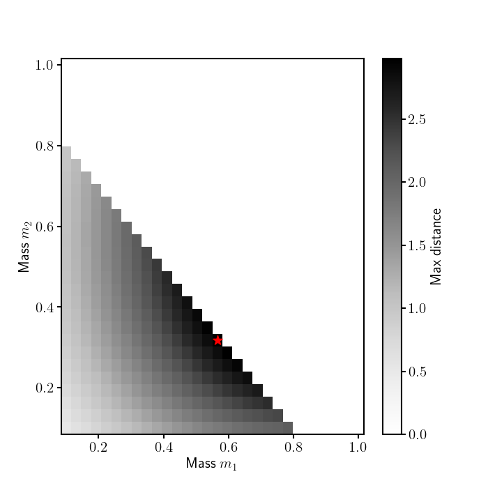
With these new masses the maxiumum distance is around $3m$ which is considerably higher than our first result.

We could also analyze the best combination of lengths $l_*$ and masses $m_*$ that maximize the distance, however I don’t think it’s going to add a lot of value to the study so I’ll leave the analysis as it is now.